05 Hydrogeochemistry and Contaminant Transport

05-06 Reactive Solute Transport

Coupling of chemical reactions with physical transport processes; conceptual and quantitative understanding of reaction fronts, plume evolution, and spatial–temporal geochemical changes.

Index	Description
05-06-001	Mass balance for a decay chain - Decay of Species A to B and species B to C
05-06-002	Analytical solution for 2D instantaneous solute transport injection in porous media (with decay)

05-06-001Mass balance for a decay chain - Decay of Species A to B and species B to C

Type: Streamlit app

Time: 5–15 min

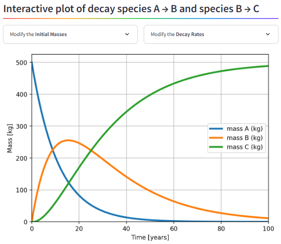
Mass balance for a decay chain - Decay of Species A to B and species B to C

Figure 1: The interactive plot of the mass balance for radioactive decay. (Screenshot)

This interactive app illustrates the mass balance of a simple decay chain (A → B → C) using a time-discrete numerical approach. It demonstrates how the decay of one species leads to the production of subsequent species while conserving total mass.

Users can modify initial masses and decay rates and explore the temporal evolution of all three species through interactive plots. The example is motivated by radioactive decay but is formulated generically, making it applicable to a wide range of first-order transformation processes relevant to hydrogeochemistry and reactive solute transport.

The app is primarily intended as a conceptual teaching tool to support the understanding of coupled decay and production processes, mass conservation, and dynamic system behavior in environmental and groundwater-related contexts.

LAUNCH RESOURCE

Detail	Value
URL	radioactive-decay.streamlit… · open app
Author(s)	Thomas Reimann (TU Dresden, Institute for Groundwater Management); Rudolf Liedl (TU Dresden, Institute for Groundwater Management)
Keywords	solute transport, decay, half-time, reactive transport, mass balance
Fit For	self learning, classroom teaching, online teaching
Prerequisites	basic chemistry

Streamlit app details

Detail	Value
Interactive plots	1 interactive plot(s)

05-06-002Analytical solution for 2D instantaneous solute transport injection in porous media (with decay)

Type: Jupyter Notebook

Time: 30–45 minutes

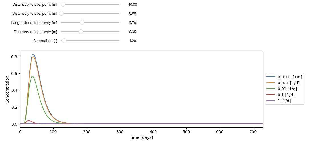
Analytical solution for 2D instantaneous solute transport injection in porous media (with decay)

Figure 1: Concentration vs. Time for five decay rates with selected parameter values. (Screenshot)

This interactive Jupyter tool computes and visualizes the analytical 2-D instantaneous solute injection solution with first-order decay in porous media. It simulates how concentration evolves over time at a given observation point for five contaminants, each defined by a different decay rate. The model incorporates:

1) Retardation
2) Longitudinal and transversal dispersion
3) Decay
4) 2-D spreading of an instantaneous point source

The user can interactively modify:

1) Distance to the observation point (x, y)
2) Longitudinal and transversal dispersivities
3) Retardation factor

The tool then automatically recalculates:

1) Effective velocity
2) Effective longitudinal and transverse dispersion
3) Time-dependent concentration curves

and plots the concentration–time profiles for all decay rates, allowing easy comparison of attenuation behavior in 2-D groundwater flow.