05 Hydrogeochemistry and Contaminant Transport
05-05 Conservative Solute Transport Processes
Physical mass-transport mechanisms: advection, mechanical dispersion, diffusion with storage, plug-flow and spreading processes; fundamental transport equations (without chemical reactions).
Contents
| Index | Description |
|---|---|
| 05-05-001 | Analytical solution for 1D continuous solute transport injection in porous media (without decay) |
| 05-05-002 | Principle of Superposition |
| 05-05-003 | 1D Transport with advection and dispersion |
05-05-001Analytical solution for 1D continuous solute transport injection in porous media (without decay)
| Type: Jupyter Notebook | Time: 30–45 minutes |
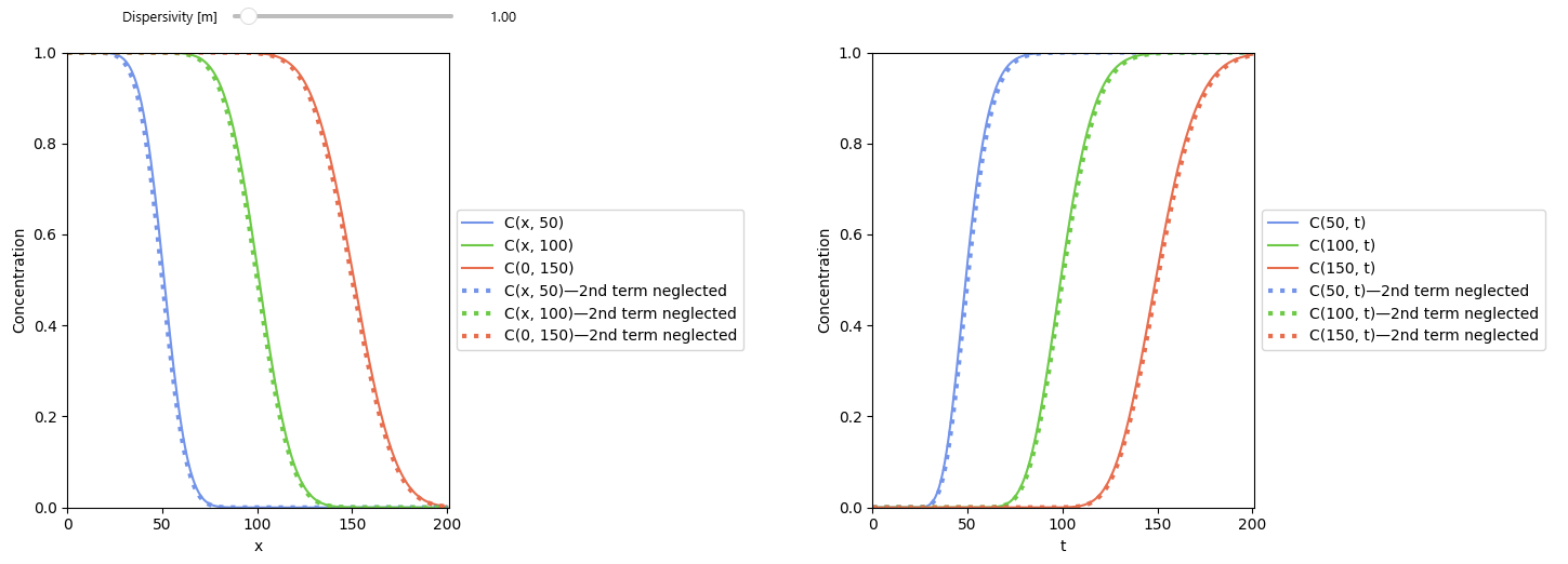
Figure 1: Evolution of the concentration in space and time with selected dispersivity values. (Screenshot)
This notebook presents the analytical 1-D solution for continuous solute transport in porous media without decay, following the classical formulation of Ogata & Banks (1961).
Using the hydrodynamic dispersion coefficient and the dimensionless Péclet number, it evaluates solute concentrations as a function of space and time under purely advective–dispersive transport. The core equation includes two terms, one representing forward transport and the other accounting for upstream dispersion.
The notebook explores when the second term becomes negligible depending on dispersivity, providing insight into advection-dominated versus dispersion-dominated regimes.
Interactive widgets allow users to dynamically adjust parameters such as dispersivity, initial concentration, time, and the groundwater velocity to visualize their impact on concentration profiles. The notebook generates breakthrough curves and spatial concentration distributions, compares full and simplified analytical solutions, and examines contaminant arrival at an observation point. It serves as an intuitive tool for understanding fundamental 1-D transport processes in groundwater systems while reinforcing key concepts from classic hydrogeology literature.
| Detail | Value |
|---|---|
| URL | github.com · open repository |
| Author(s) | Oriol Bertran (UPC); Daniel Fernàndez-Garcia (UPC) |
| Keywords | analytical solutions, solute transport, continuous injection, 1D, no decay |
| Fit For | self learning, online teaching, classroom teaching |
| Prerequisites | None specified. |
Images
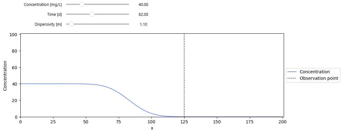
Figure 2: Evolution of the concentration in space with selected parameter values. (Screenshot)
05-05-002Principle of Superposition
| Type: Jupyter Notebook | Time: 30–45 minutes |
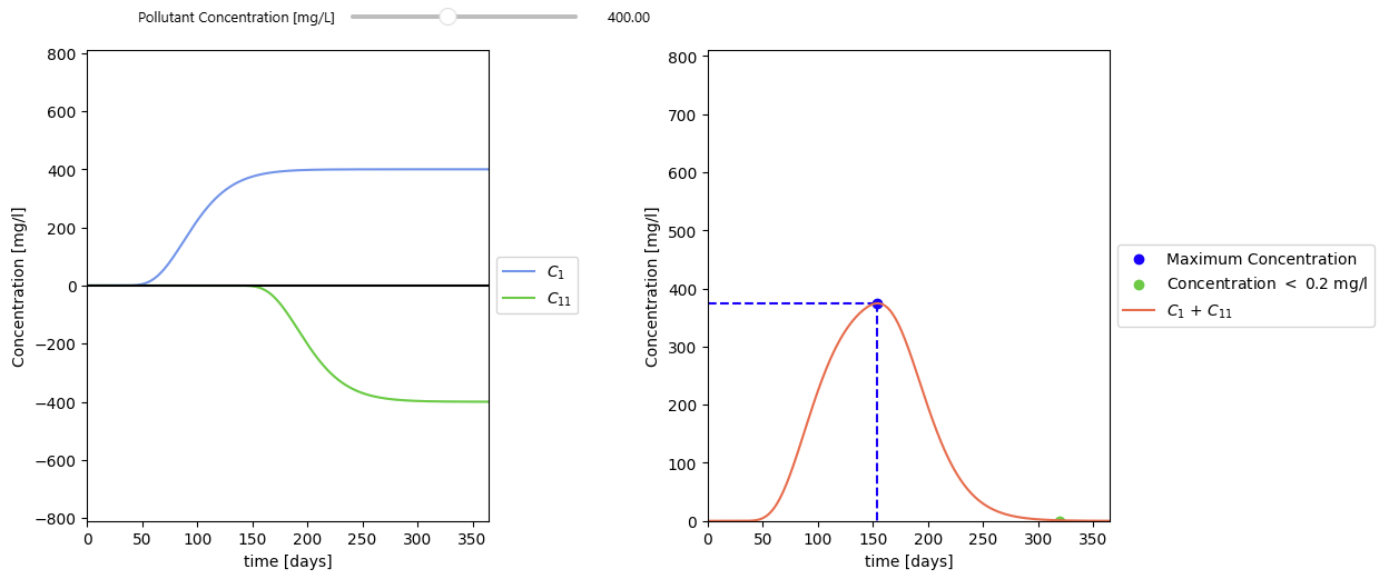
Figure 1: Pulse injection (Screenshot)
This notebook demonstrates the principle of superposition applied to one-dimensional solute transport in porous media. Since the advection–dispersion equation is linear in concentration, individual concentration contributions from different sources or release events can be added to obtain the total solution.
The notebook first defines the governing transport equation for continuous injection without decay, using the classical Ogata–Banks analytical solution. It then sets up helper functions for dispersion, the Péclet number, and concentration calculations, along with interactive widgets that allow the user to modify input parameters and visually explore how multiple releases combine.
Two practical examples illustrate how superposition works in groundwater contamination scenarios. In the first example, two overlapping continuous releases—one starting at time zero and another beginning later—are simulated independently and then added to obtain the combined breakthrough curve at an observation point.
In the second example, a pulse injection is represented by subtracting two continuous injections, showing how a short-duration spill can be reconstructed using linearity. Interactive plots reveal the timing, peak concentration, and dissipation behavior of each scenario, giving users an intuitive understanding of how linear transport processes respond to multiple or time-varying sources.
| Detail | Value |
|---|---|
| URL | github.com · open repository |
| Author(s) | Oriol Bertran (UPC); Daniel Fernàndez-Garcia (UPC) |
| Keywords | solute transport, principle of superposition |
| Fit For | self learning, online teaching, classroom teaching |
| Prerequisites | None specified. |
Images
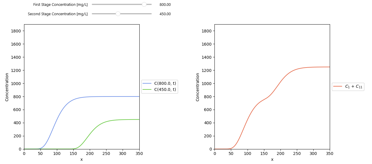
Figure 2: Continuous injection (Screenshot)
05-05-0031D Transport with advection and dispersion
| Type: Streamlit app | Time: 15–30 minutes |
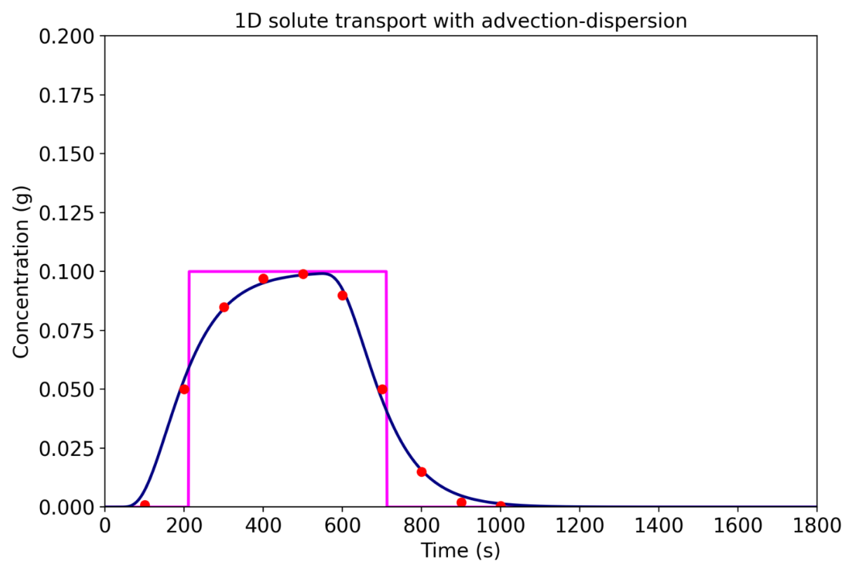
Figure 1: The computed breakthrough curve for 1D advective-dispersive transport, together with (Screenshot)
This interactive app illustrates one-dimensional solute transport under steady groundwater flow, focusing on the combined effects of advection and longitudinal dispersion. A finite-duration pulse input is applied at the source, and the app computes and plots the resulting breakthrough curve (concentration versus time) at a user-defined observation distance.
Users can vary key transport parameters such as porosity and longitudinal dispersivity, and compare alternative representations by toggling between advection-only transport and the advection–dispersion solution. An optional set of example measurements can be displayed for visual comparison with the simulated breakthrough curve. The app supports conceptual understanding of plume spreading, travel times, and parameter sensitivity in 1D transport problems and is suited for teaching and self-study in hydrogeology and contaminant transport.
| Detail | Value |
|---|---|
| URL | transport-1d-ad.streamlit.a… · open app |
| Author(s) | Thomas Reimann (TU Dresden); Rudolf Liedl (TU Dresden) |
| Keywords | solute transport, advection, dispersion, analytical solution |
| Fit For | self learning, online teaching, classroom teaching |
| Prerequisites | Basic hydrogeology, Aquifer parameters |
Streamlit app details
| Detail | Value |
|---|---|
| Interactive plots | 1 interactive plot(s) |