08 Groundwater Modeling
08-02 Numerical Schemes
Spatial/temporal discretization, stability, solution algorithms, convergence.
Contents
| Index | Description |
|---|---|
| 08-02-001 | Finite Difference Numerical Scheme |
| 08-02-002 | Finite-Difference Numerical scheme: Solver options |
08-02-001Finite Difference Numerical Scheme
| Type: Streamlit app | Time: 15–30 minutes |
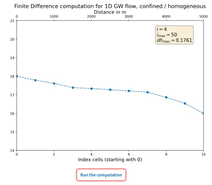
Figure 1: The interactive plot with the basic setup. When the computation is running, the shown head values update. (Screenshot)
Purpose and Functionality The app implements the one-dimensional finite difference method for groundwater flow with two fixed head boundary conditions. Users can specify the spatial discretization by selecting the number of cells, upon which the numerical scheme is set up and solved.
Learning Features The app visualizes the iterative development of the numerical solution and illustrates how the approximation approaches a stable state. A built-in analytical reference solution enables direct comparison, supporting the exploration of error behaviour, convergence, and numerical representation of groundwater flow processes.
| Detail | Value |
|---|---|
| URL | gwf-1d-conf-fd.streamlit.app · open app |
| Author(s) | Thomas Reimann (TU Dresden); Rudolf Liedl (TU Dresden) |
| Keywords | Numerical solution, groundwater modeling, applied hydrogeology, finite differences |
| Fit For | self learning, online teaching, classroom teaching |
| Prerequisites | Basic hydrogeology, 1D groundwater flow equation, analytical solutions for 1D groundwater flow, |
Streamlit app details
| Detail | Value |
|---|---|
| Interactive plots | 1 interactive plot(s) |
Images
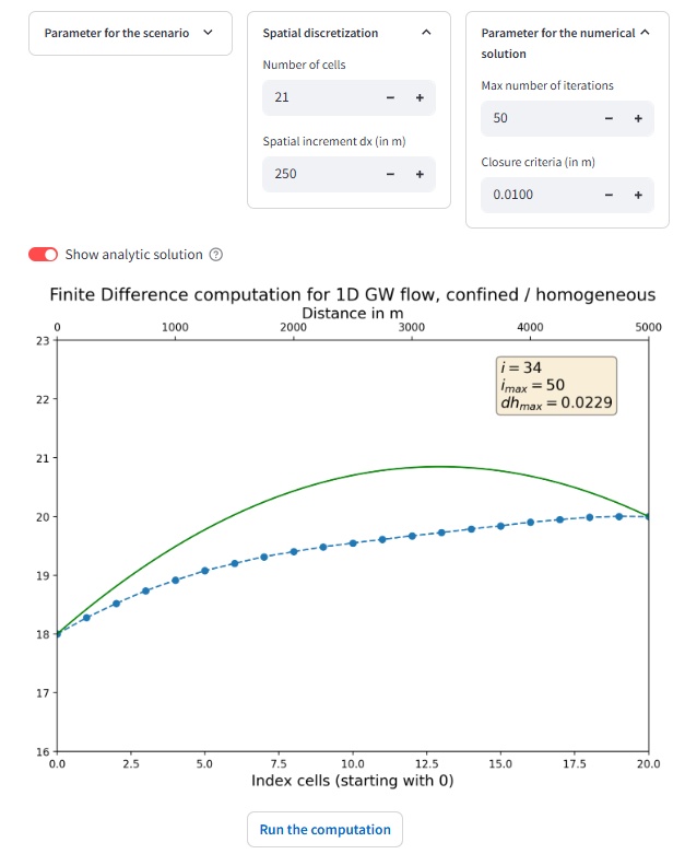
Figure 2: The user interface with an interactive plot that comes with an modified spatial discretization. In addition, the analytical solution is show that allows students comparison with the numerical results. (Screenshot)
08-02-002Finite-Difference Numerical scheme: Solver options
| Type: Streamlit app | Time: 15–30 minutes |
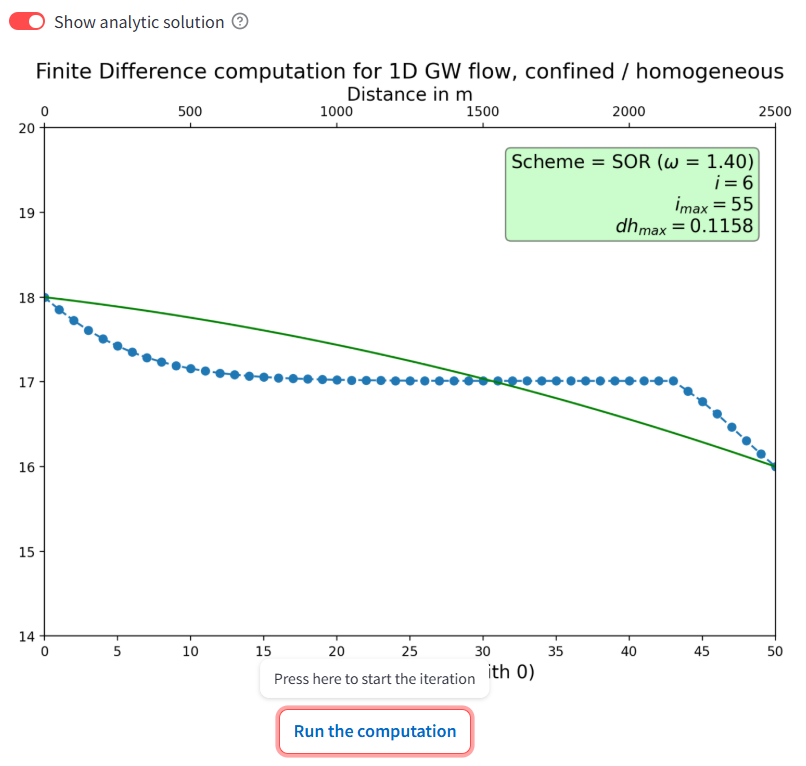
Figure 1: The interactive plot shows the development of the solution. Various solver options (Screenshot)
This app illustrates the numerical solution of the 1D groundwater flow equation for a confined aquifer using a finite-difference scheme. Users can interactively compare Jacobi, Gauss–Seidel, and SOR solvers, visualize the iterative path toward convergence, and evaluate results against the analytical solution. The tool supports conceptual understanding of solver behavior, convergence characteristics, and numerical accuracy in groundwater modeling.
| Detail | Value |
|---|---|
| URL | gwf-1d-conf-fd-solvers.stre… · open app |
| Author(s) | Thomas Reimann (TU Dresden) |
| Keywords | 1D flow, finite differences, solver, solution schemes, SOR, Gauss-Seidel, Jacobi |
| Fit For | self learning, classroom teaching, online teaching |
| Prerequisites | Basic hydrogeology, groundwater flow equation |
Streamlit app details
| Detail | Value |
|---|---|
| Interactive plots | 1 interactive plot(s) |